Obrazowanie „magnetyczne” w medycynie

Prezentacja na temat: "Obrazowanie „magnetyczne” w medycynie"— Zapis prezentacji:

1 Obrazowanie „magnetyczne” w medycynie
Badanie rozkładu pola magnetycznego generowanego przez prądy – diagnostyka mózgu i serca Badanie magnetyczne przewodu pokarmowego Termoterapia za pomocą pola zmiennego Termoterapia za pomocą cząstek magnetycznych B. Augustyniak

2 Natężenia pola magnetycznego w środowisku
Natężenia pola magnetycznego dla różnych źródeł oraz zakresy czułości mierników pola Magnetism in Medicine – Handbook; WILEY-VCH Verlag GmbH, Weinheim, 2007 B. Augustyniak

3 Pola magnetyczne i sygnały MEG
Several selected channels of an MEG measurement are displayed in the insets. They show how artefacts like the subject’s heart beat, eye blinks, and spontaneous alpha rhythm may severely disturb the monitoring of the much smaller brain activity A typical averaged event-related signal is displayed in the bottom panel. B. Augustyniak Journal of Low Temperature Physics, Vol. 146, Nos. 5/6, March 2007

4 Rozdzielczość x-t metod obrazowania
B. Augustyniak Journal of Low Temperature Physics, Vol. 146, Nos. 5/6, March 2007

5 Badania rozkładów pola magnetycznego generowanego przez prądy płynące lokalnie w ciele
Magnetoencephalography MEG B. Augustyniak

6 Źródła pola magnetycznego w głowie
The MEG (and EEG) signals derive from the net effect of ionic currents flowing in the dendrites of neurons during synaptic transmission. B. Augustyniak

7 Komórki nerwowe brain.fuw.edu.pl/~suffa/SygnalyBioelektryczne/Sygnaly1.ppt

8 Warunki powstania efektywnego pola amagnetycznego od neronów
In order to generate a signal that is detectable, approximately 50,000 active neurons are needed. Since current dipoles must have similar orientations to generate magnetic fields that reinforce each other, it is often the layer of pyramidal cells in the cortex, which are generally perpendicular to its surface, that give rise to measurable magnetic fields. Furthermore, it is often bundles of these neurons located in the sulci of the cortex (kora) with orientations parallel to the surface of the head that project measurable portions of their magnetic fields outside of the head. B. Augustyniak

9 Historia MEG The MEG was first measured by David Cohen in 1968, before the availability of the SQUID, using only a copper induction coil as the detector. To reduce the magnetic background noise, the measurements were made in a magnetically shielded room. However, the insensitivity of this detector resulted in poor, noisy MEG signals, which were difficult to use. Then, later at MIT, he built a better shielded room, and used one of the first SQUID detectors (just developed by Zimmerman) to again measure the MEG This time the signals were almost as clear as the EEG, and stimulated the interest of physicists who had begun looking for uses of SQUIDs. Thus, the MEG began to be used, so that various types of spontaneous and evoked MEG’s began to be measured. At first only a single SQUID detector was used, to successively measure the magnetic field at a number of points around the subject’s head. This was cumbersome, and in the 1980’s, MEG manufacurers began to increase the number of sensors to cover a larger area of the head, using a correspondingly larger dewar. Present-day MEG dewars are helmet-shaped and contain as many as 300 sensors, covering most of the head, as shown in the first figure. In this way, MEG’s of a subject or patient can now be accumulated rapidly and efficiently. B. Augustyniak

10 MEG typu ‘Magnes 3600 WH’ B. Augustyniak
Magnetism in Medicine – Handbook; WILEY-VCH Verlag GmbH, Weinheim, 2007, Journal of Low Temperature Physics, Vol. 146, Nos. 5/6, March 2007 B. Augustyniak

11 Schemat detektorów SQUID
The picture shows the sensor arrangement of the Elekta Neuromag 306 whole-head system B. Augustyniak

12 Fazy badania MEG 1 Impuls elektryczny płynący przez neuron – generacja impulsu pola magnetycznego B. Augustyniak

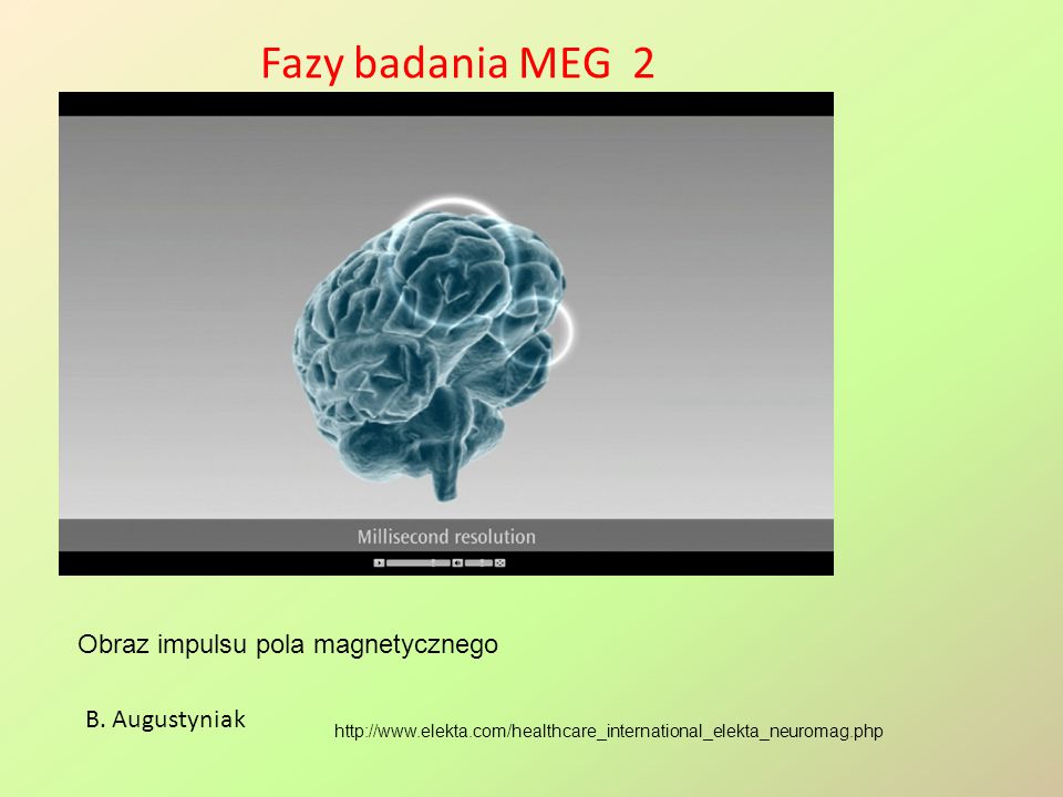
13 Fazy badania MEG 2 Obraz impulsu pola magnetycznego B. Augustyniak

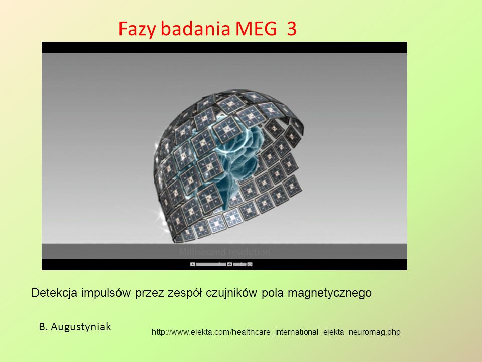
14 Fazy badania MEG 3 Detekcja impulsów przez zespół czujników pola magnetycznego B. Augustyniak

15 Detale układu MEG ze SQUID
Cutaway drawing of the „Magnes” dewar showing the location of the reference channels relative to the sensor coils B. Augustyniak

16 Matryca czujniki SQUID
B. Augustyniak

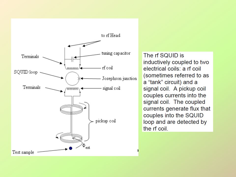
17 SQUID Superconducting Quantum Interference Device
Jak to działa ? Bolesław AUGUSTYNIAK

18 Strumień pola magnetycznego przez nadprzewodzącą pętlę
Prąd płynie po powierzchni nadprzewodnika wytwarzając strumień Fsc. Kwant strumienia Fo to flukson B. Augustyniak Wstęp do fizyki ciała stałego; Ch. Kittel, PWN, Warszawa, 1999

19 Tunelowanie elektronów przez złącze przewodnik-izolator-przewodnik
Dwa przewodniki A i B oddzielone warstwą izolatora C o grubości rzędu 10 A. Po oziębieniu jeden z przewodników staje się nadprzewodnikiem Dla złącza z nadprzewodników w bardzo niskiej temperaturze nie może płynąć prąd o ile napięcie nie przekroczy wartości Vc = Eg/2e, gdzie Eg jest przerwą energetyczną między pasmami walencyjnym i przewodnictwa B. Augustyniak Wstęp do fizyki ciała stałego; Ch. Kittel, PWN, Warszawa, 1999

20 Złącze Josephsona dla nadprzewodników
Następuje tunelowanie par Coopera przez cienką barierę pomiędzy nadprzewodnikami. Można obserwować dwa zjawiska Josephosna: 1. stałoprądowe (prąd stały płynie przez złącze bez zewnętrznego napięcia) 2. zmiennoprądowe (stałe napięcie przyłożone do złącza powoduje oscylacje natężenia prądu płynącego przez złącze B. Augustyniak

21 Stałoprądowe zjawisko Josephsona
funkcje falowe Y1 i Y2 pary po obu stronach złącza n1 i n2 – ‘koncentracje’ nośników Natężenie J prądu stałego może mieć różne wartości, zależnie od różnicy faz d funkcji falowych Y1 i Y2 po obu stronach złącza Prądu Jo jest maksymalnym prądem dla U = 0 B. Augustyniak Wstęp do fizyki ciała stałego; Ch. Kittel, PWN, Warszawa, 1999

22 Zmiennoprądowe zjawisko Josephsona
Po przyłożeniu różnicy potencjałów V do złącza zmienia się energia par po obu stronach złącza a także zmienić się zaczyna w czasie różnica faz funkcji falowych, tym szybciej, im większe jest napięcie V Płynący prąd staje się prądem przemiennym !!! Napięcie na złączu V = 1 mV wywołuje oscylacje o częstości 483,6 MHz!!! B. Augustyniak Wstęp do fizyki ciała stałego; Ch. Kittel, PWN, Warszawa, 1999

23 DC Josephson : A dc current flows across the junction in the absence of
any electric or magnetic field. AC Josephson : A dc voltage applied across the junction causes rf current oscillations across the junction. This effect has been utilized in a precision determination of the value of Further, an rf voltage applied with the dc voltage can then cause a dc current across the junction. Macroscopic long-range quantum interference: A dc magnetic field applied through a superconducting circuit containing two junctions causes the maximum supercurrent to show interference effect as a function of magnetic field intensity. Magnetometer

24 Pętla z dwoma złączami Josephsona w polu magnetycznym B
Przez pętle przepuszcza się prąd o natężeniu J przy U = 0. Strumień magnetyczny F = B *S zmienia fazy funkcji falowych par Coopera płynących w gałęziach a i b Prąd J jest sumą prądów z obu gałęzi Natężenie prądu jest periodyczną funkcją strumienia F. Maksima występują dla warunku , s – liczba całkowita B. Augustyniak Wstęp do fizyki ciała stałego; Ch. Kittel, PWN, Warszawa, 1999

25 Oscylacje natężenia prądu dla pętli z dwoma złączami Josephsona w polu magnetycznym B
B. Augustyniak Wstęp do fizyki ciała stałego; Ch. Kittel, PWN, Warszawa, 1999

26 SQUID: ZASADA DZIAŁANIA - 2
Prąd I wchodząc do pierścienia rozdziela się na dwa prądy, których fazy zależą od strumienia pola magnetycznego ww. i które interferują A IA=I0sinA A-B=/0 I A maksymalny prąd nadprzewodzący który może płynąć przez złącze oscyluje; oscylacje zależą od pola B wewnątrz pierścienia  1 2 B I=IA+IB Jeśli przez złącze przepuszczony jest prąd większy, to nadwyżka wytwarza napięcie B IB=I0sinB Amplituda prądu nadprzewodzącego Napięcie oscyluje z okresem 0 (n+1/2) I W DC SQUIDzie plynacy prad rozdziela się na 2, przez gorne i dolne zlacze, inne, w zaleznosci od roznicy faz funkcji po obu stronach zlacza. Ta roznica faz, z kolei zalezy od strumienia pola magnetycznego przeplywajacego przez obszar petli. Prady interferuja prowadzac do analogicznego zjawiska jak interferencja na dwoch szczelinach. Mianowicie, amplituda stalego pradu nadprzewodzacego, czyli takiego dla którego napiecie na zlaczach jest zero zmienia się. Jeśli teraz przez SQUIDa przepuscimy prad troche wiekszy niż maksymalny, to pojawi się napiecie, ale zalezne od tego jak nasz prad jest wiekszy od maksymalnego prady nadprzewodzacego. A ten się zmienia, wiec zmienia się tez napiecie. I to napiecie możemy obserwowac. Tyle oscylacji napiecia, ile kwantow strumienia jest w pierscieniu. Niezaleznie od typu przez pomiar zmian napiecia możemy wnioskowac o strumieniu przez pierscienie, czyli o polu magnetycznym. Co prawda czulosci sa zblizone, ale dawniej latwosc konstrukcji przemawiala za RF SQUIDem, a teraz DC SQUID jest czulszy i czesciej uzywany. Konstruuje się również SQUIDy na nadprzewodnikach wysokotemperaturowych. n I0 V Czułość 10V/0 -1 1 /0 V Nowe techniki.ppt

27 Magnetometry ze SQUID B. Augustyniak

28 Pomiar pól zmiennych poprzez sprzężenie z pętlą SQUID
A magnetometer measures the magnitude of an applied magnetic field. In this case, the flux transformer is a simple two-coil DC transformer. Normally both the pickup and secondary coils are superconducting and therefore need to be cooled. The pick-up coil is placed in the field to be measured, causing a field to be set up by the secondary coil, which in turn is detected by the SQUID L1 - Pick-up coil – cewka pomiarowa L2 – secondary (input) coil – cewka sprzęgająca – wytwarza wtórny stumień B. Augustyniak

29 C. P. Sun, National Sun Yat Sen University

30 C. P. Sun, National Sun Yat Sen University

31

32 MEG - Badanie pola magnetycznego mózgu
Magnes 3600 WH in position for a seated study. Magnetism in Medicine – Handbook; WILEY-VCH Verlag GmbH, Weinheim, 2007 B. Augustyniak

33 Impulsy ‘magnetyczne’ od impulsów w neuronach
B. Augustyniak

34 Sygnały MEG -epilepsja
B. Augustyniak

35 Sygnały z czujników pola magnetycznego
Waveform, field distribution and source localization data for 13-month-old infant with infantile spasms studied with conscious sedation. The patient was positioned with her head centered in the sensor array of a Magnes 2500 WH 148-channel system. Magnetism in Medicine – Handbook; WILEY-VCH Verlag GmbH, Weinheim, 2007 B. Augustyniak

36 Badanie akcji mózgu systemem VSM MedTech
(a) Cortical 275-channel CTF MEGTM System (VSM MedTech). (b) MEG of a somatosensory-evoked field recorded by CTF MEGTM System (DC to 300 Hz bandwidth, 628 averages and third-order gradiometer noise cancellation). Magnetism in Medicine – Handbook; WILEY-VCH Verlag GmbH, Weinheim, 2007 B. Augustyniak B. Augustyniak

37 Lokalizacja ‘muzyki’ B. Augustyniak
Left:(MEG-based brain surface current density (BSCD) reconstructions of motor activity in musicians listening to piano music (Haueisen and Knosche, 2001). Magnetism in Medicine – Handbook; WILEY-VCH Verlag GmbH, Weinheim, 2007 B. Augustyniak

38 SQUID - badanie mózgu myszy !
9-channel magnetometer array probe with low noise and high spatial resolution for magnetocardiograph (MCG) measurements of mice and rats. The magnetometer based on a low-Tc superconducting interference device (SQUID) has a circular pickup loop with the diameter of 2.5 mm and is arrayed in a 3×3 matrix with the spatial interval of 2.75 mm on a 10 mm×10 mm silicon chip. Overviews of the fabricated SQUID magnetometer array. A bare SQUID magnetometer array chip (a), flipchip connection on a substrate (b), and protection with an epoxy resin (c). B. Augustyniak International Congress Series 1300 (2007) 570–573

39 SQUID - badanie mózgu myszy 2
A SQUID magnetometer array probe B. Augustyniak International Congress Series 1300 (2007) 570–573

40 SQUID - badanie mózgu myszy 3
Real-time MCG signals recorded with a mouse using the SQUID magnetometer array. The upper-right is the averaged waveforms. B. Augustyniak International Congress Series 1300 (2007) 570–573

41 MEG - podsumowanie Od lat 1980, pomiary pola magnetycznego za pomocą wielu (~300) nadprzewodzących detektorów SQUID (wymagają ciekłego helu). Tło jest rzędu 108 fT, sygnały mózgu rzędu 10 fT. MEG wymaga pobudzenia ~ neuronów, wykrywa prądy. Główne zastosowania to analiza ognisk padaczki, określanie obszarów kory przetwarzającej sygnały zmysłowe, funkcje językowe. Zalety: Wysoka rozdzielczość czasowa (<1 ms). Dociera do głębszych struktur (ale tylko podłużne prądy). Wady: Wysoka cena, skomplikowane urządzenie. Mała rozdzielczość przestrzenna przy identyfikacji źródeł (5 cm). Trudności interpretacyjne. B. Augustyniak

42 Magnetyczne obrazowanie serca
B. Augustyniak

43 Magnetyczne obrazowanie serca (MCG)
B. Augustyniak

44 Magnetyczne obrazowanie serca (MCG)
The similarity between the lead fields of certain electric and magnetic leads are illustrated. If the magnetic field is measured in such an orientation (in the x direction in this example) and location, that the symmetry axis is located far from the region of the heart, the magnetic lead field in the heart's region is similar to the electric lead field of a lead (lead II in this example), which is oriented normal to the symmetry axis of the magnetic lead. B. Augustyniak

45 Magnetyczne obrazowanie serca (MCG)
Symmetric XYZ lead system. The bipolar arrangement provides good lead field uniformity. The difficulty arises in locating all magnetometers in their correct position surrounding the body. . B. Augustyniak

46 Magnetyczne obrazowanie serca (MCG)
Symmetric XYZ lead system. The bipolar arrangement provides good lead field uniformity. The difficulty arises in locating all magnetometers in their correct position surrounding the body. . Realization of the unipositional lead system. The arrows indicate the measurement direction. The shaded sphere represents the heart B. Augustyniak

47 Magnetyczne obrazowanie serca (MCG)
Schematic illustration of the generation of the x component of the MCG signal. The source of the MCG signal is the electric activity of the heart muscle. As regards the x component, it is assumed that because of the strong proximity effect, the signal is generated mainly from the activation in the anterior part of the heart B. Augustyniak

48 Magnetyczne obrazowanie serca (MCG)
Averaged MHV recorded with the unipositional lead system B. Augustyniak

49 Badania magnetyczne pracy serca
Locus of the total current dipole vector, P, during the cardiac cycle and magnetocardiogram in a healthy subject. Signal-averaged traces from a 61-channel prethoracic acquisition. Magnetic field map at Q onset schematically superimposed on an MR image. Magnetism in Medicine – Handbook; WILEY-VCH Verlag GmbH, Weinheim, 2007 B. Augustyniak

50 Diagnostyka magnetyczna przewodu pokarmowego za pomocą śledzenia ruchu „magnetycznych” elementów

51 Badania magnetyczne pracy przewodu pokarmowego
PTB 83-SQUID system. (a) Path of the magnetically marked dosage form through the GI tract of a volunteer in the fasted state. PTB 83-SQUID system. (a) system inside the shielded room SQUID, (b) S configuration (top view); Magnetism in Medicine – Handbook; WILEY-VCH Verlag GmbH, Weinheim, 2007 B. Augustyniak

52 Thermoterapia magnetyczna
Wykorzystanie prądów wirowych Wykorzystanie cząstek magnetycznych

53 1. Magnetoterapia za pomocą zmiennego pola magnetycznego
Generator prądu (a) i aplikatory (b) (cewki szpulowe) przykładowego urządzenia do magnetoterapii B. Augustyniak Praca naukowo-badawcza z zakresu prewencji wypadkowej, CIOP, 2008

54 Thermoterapia z wykorzystaniem ogrzewania cząsteczek magnetycznych wymuszonego zmiennym polem magnetycznym

55 2. Termoterapia za pomocą cząsteczek magnetycznych
Frequency dependence of temperature rise for ferrite powders after an application of AC magnetic field for 2 min: Core loss for ferrite powder as function of frequency at room temperature ð25CÞ under HAC ¼ 30 A=m: Nanoparticles in photodynamic therapy: An emerging paradigm; Advanced Drug Delivery Reviews Volume: 60, Issue: 15, December 14, 2008, pp ; Chatterjee, Dev Kumar; Fong, Li Shan; Zhang, Yong B. Augustyniak

56 Termoterapia za pomocą pola f =100 kHz i płynów magnetycznych
Sketch of the first prototype MFH therapy system (MFH Hyperthermiesysteme GmbH,Berlin,Germany). The AC magnetic field axis is perpendicular to the axial direction of the patient couch (1). The therapy system is for universal application, i.e., suitable for MFH within, in principle, any body region. It is a ferrite-core applicator (2) operating at a frequency of 100 kHz with an adjustable vertical aperture of cm (3). The field strength is adjustable from 0 to 15 kA/m. The system is air cooled (4). Presentation of a new magnetic field therapy system for the treatment of human solid tumors with magnetic fluid hyperthermia , Journal of Magnetism and Magnetic Materials Volume: 225, Issue: 1-2, 2001, pp Jordan, A.; at all B. Augustyniak

57 Termoterapia za pomocą pola zmiennego
3D field strength distributions were calculated using the ‘finite-difference-time-domain-(FDTD)-method‘ . One example of the visualized results is shown in Fig. 3A (3D vector diagram, coronary view,24 cm aperture, 15 kA/m) Presentation of a new magnetic field therapy system for the treatment of human solid tumors with magnetic fluid hyperthermia; Journal of Magnetism and Magnetic Materials Volume: 225, Issue: 1-2, 2001, pp Jordan, A et. al. B. Augustyniak