Włodzimierz Godłowski

Prezentacja na temat: "Włodzimierz Godłowski"— Zapis prezentacji:

1 Włodzimierz Godłowski
ON THE ORIGIN OF LARGE SCALE STRUCTURES Piotr Flin Włodzimierz Godłowski Elena Panko Instytut Fizyki, Uniwersytet Jana Kochanowskiego, Kielce, Polska Instytut Fizyki, Uniwersytet Opolski, Opole, Polska Kalinenkov Astronomical Observatory, Nikolaev, Ukraine

2 Włodzimierz Godłowski
Piotr Flin Włodzimierz Godłowski Elena Panko

3 Plan Kilka uwag historycznych Obserwacje Symulacje numeryczne
Używane obserwacje: Dwa zestawy danych Grupy Tully’ego w LSC Katalog struktur PF Kształt struktur Supergromady Efekt Binggeli’ego obiekty katalogu PF obiekty NBG Konkluzje

4 Outlook A few historical remarks Observations Numerical simulations
Applied observational data: Two sets: LSC: Tully’s group w LSC Struktures catalogue PF Structure shape Superclusters Binggeli effect PF structures NBG groups Conclusions

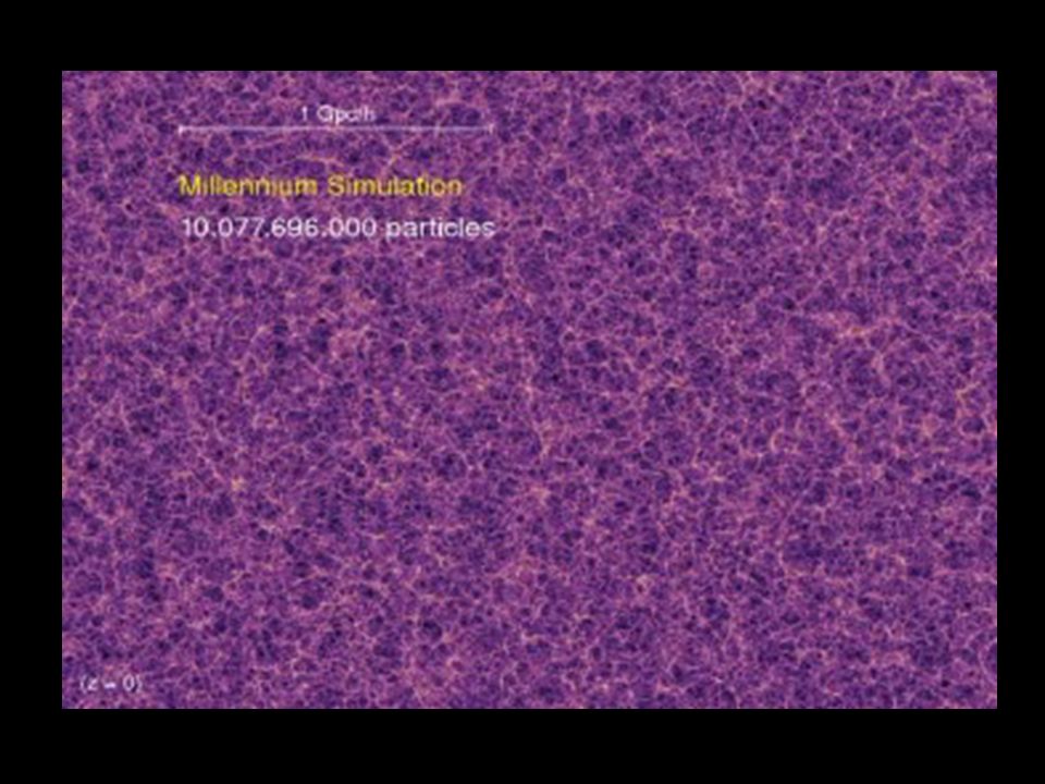
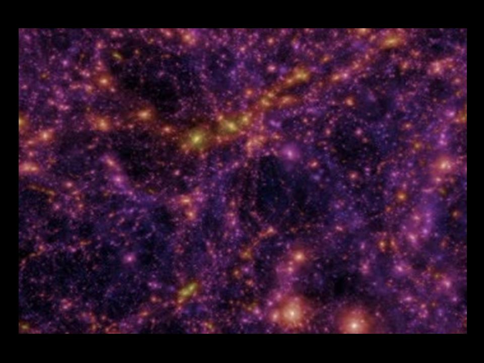
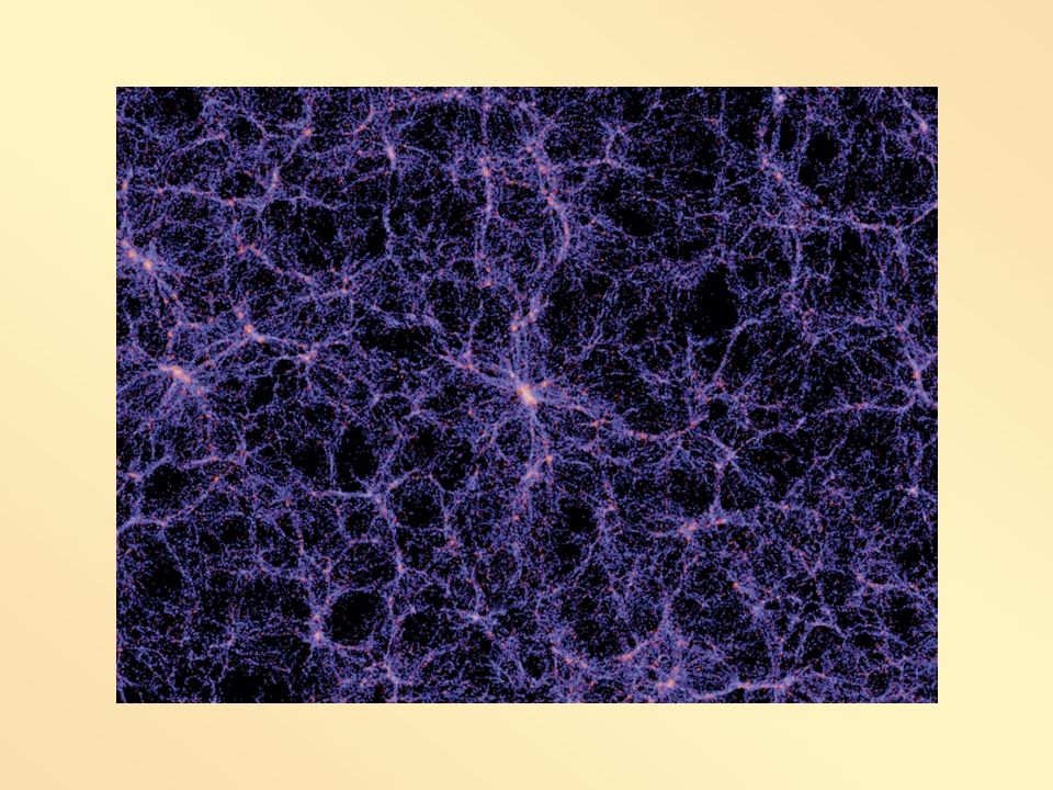
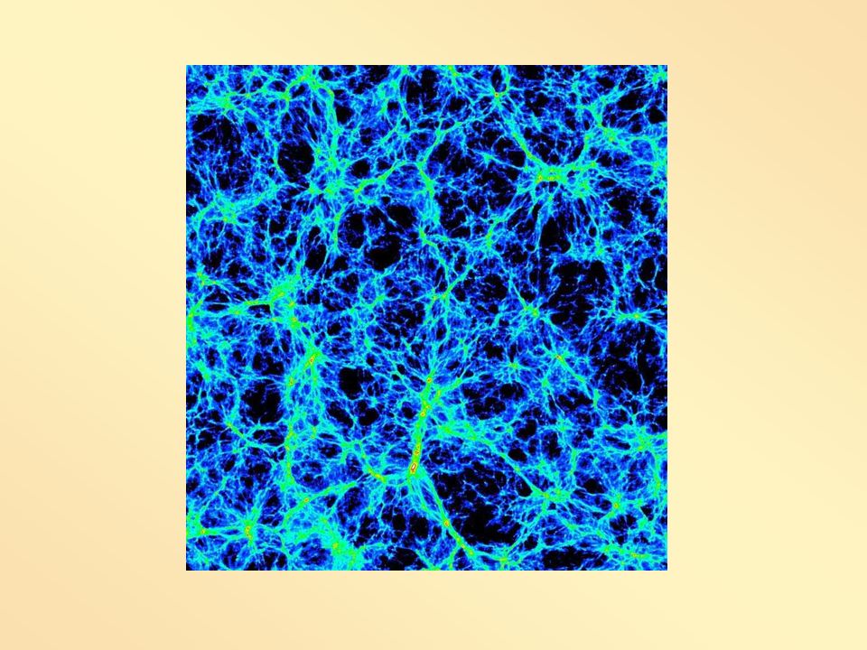
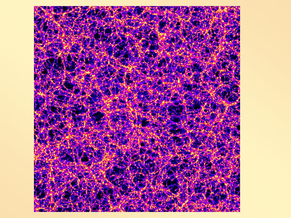
5 Large scale distribution of matter in the Universe (cosmic web)
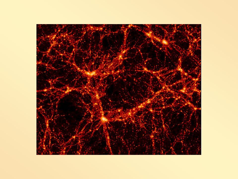
long structures (filaments) flat structures (sheets, walls) dense, compact regions (galaxy clusters ) surrounded by depopulated regions (voids)

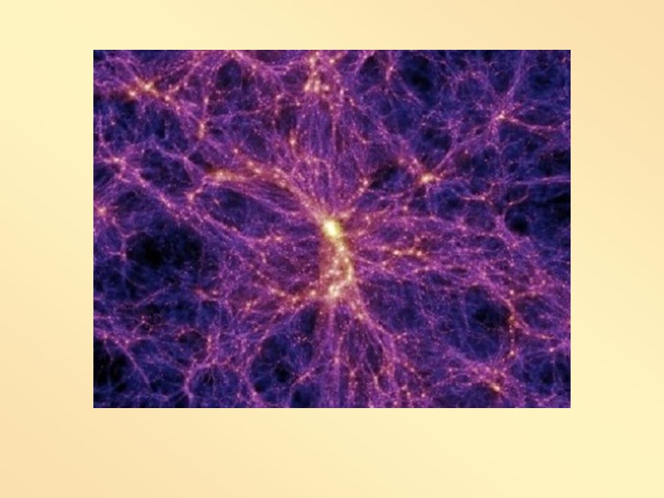
6 Cosmic web: structures and voids kosmiczna sieć : strucures and voids

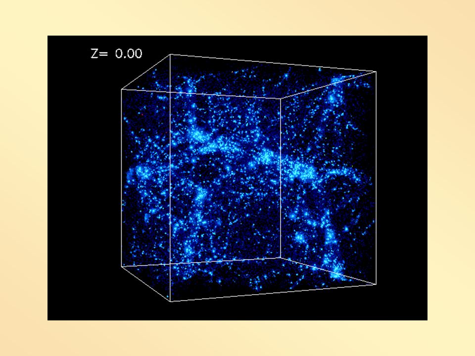
7 Cen & Ostriker (2006)

8

9 Motivation

10

11

12 LSC GF ApJ 70,.920 (2010)

13

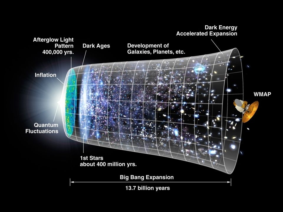
14 Considered model HOT BIG BANG EKSPANSION OF THE UNIVERSE
106 YAERS AFTER THE BIG bANG Temperature of matter and radiations ~3*103 K: primival plasma recombination free electrons disappeared, drastic reduction of the radiation and matter interactions, Independent evolution of radiation and matter. The Universe becames transparent

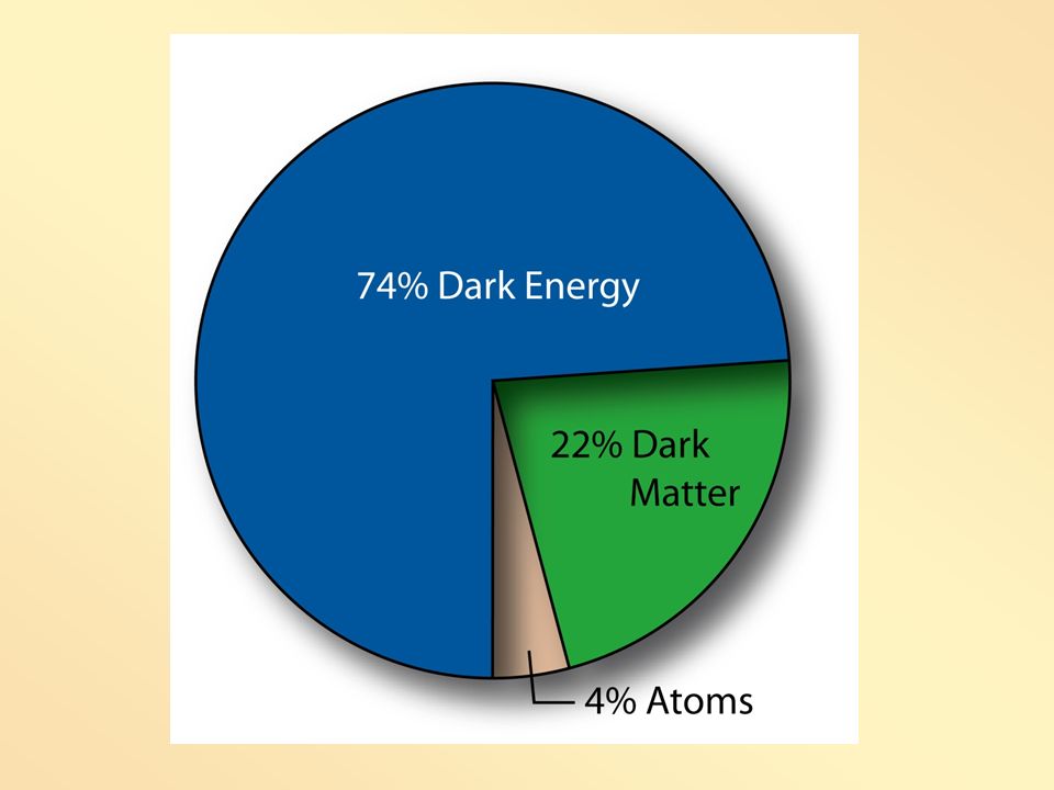
15 Kind of matter: Barionic non barionic, what is the distribution of both ? HOT : lekkie ( ~100 eV) i relatywistyczne aż do rekombinacji cząstki ( neutrino) WARM (1 – 10 keV) stają się nie- relatywistyczne wcześniej COLD ciężkie cząstki, która bardzo wcześnie przestają być relatywistyczne Mają bardzo małe prędkości Gravitinos, photinos, axions (WIMP)

16 Parameters conected with density perturbations
Type of perturbation Amplitude Skale of perturbation (MASS or the scale lenght TREE MAIN TYPES OF FLUKTUATIONS: ADIABATIC (RADIATION AND MATTER ARE PERTURBED ), (ENTROPIA PER BARION IS CONSTANT) ISOTERMIC PERTURBACJE (TEMPERATURE AND RADIATION DENSITY = CONST, ONLY MATTER FORMS AGGREGATIONS) 3. TURBULENCES (EDGGES) - (BOTH MATTER AND RADIATION) Various scenerios structure origin predicts diferent proerties of structures: mainly shape and the acquitance of angular momenta of galaxies. modele : top – down, bottom – up

17 Explosive scenario Wiele małych eksplozji równocześnie 25 – 50 Mpc
1065 erg lub Nadprzewodzące struny kosmiczne Młode galaktyki, kwazary do 5 Mpc 1061 erg

18

19

20

21

22 Hierarchical clustering (tidal torquing)
Turbulences Pancake Hierarchical clustering (tidal torquing) Iye & Sugai, 1991ApJ 374, 12

23 Observational data From Tully’s Catalogue: 61 galaxy groups
26 groups with objects >20 objects Position angle of the group PAg Position angle of the line joining 2 brightest galaxies PAl Position angle of the BCM PAbm Direction toward Vigo Cluster centre PAV Isotropy tested (K-S, c2 )

24

25

26 The distribution of the acute angle Θ between the position angle of the major axis of a given group (PAg) and direction towards other groups. From top to bottom the distributions for galaxies with D  10 Mpc, 10<D 20 Mpc, 10<D 20 Mpc and D>20 Mpc are presented respectively.

27 The distribution (from top to bottom) of the differences between position angles (PAg-PAV, PAl-PAV, PAg-PAl).

28 The distribution (from top to bottom) of the position angle of the major axis of a given group (PAg), the position of the line joining two brightest galaxies in the group (PAl) and direction towards Virgo cluster (PAV).

29 Two brightest originated on the filament directed toward the centre of of LSC.
Through the gravitational interaction galaxy groups are formed on the line conected these two brightest galaxies. Therefore we observed aligment of structure and line connecting two brightes

30

31

32

33

34

35

36

37

38 This is picture showing the origin in the case of not very massive sytucture, as LSC. It is interesting to look in greater scale and in 2D. There are not statistically complete data for such a task. Therefore, we decided to check the observed tendency. We will use the PF Catalogue .

39 Observational data The Muenster Red Sky Survey is a large-sky galaxy catalogue covering an area of about 5000 square degrees on the southern hemisphere. The catalogue includes 5.5 millions galaxies and is complete till photo-graphic magnitude rF=18m.3 (Ungruhe 2003). 217 ESO Southern Sky Atlas R Schmidt plates with galactic latitudes b<-45 were digitized with the two PDS microdensitometers of the Astronomisches Institut at Muenster. The classification of objects into stars, galaxies and perturbed objects was done with an automatic procedure with a posterior visual check of the automatic classification. The external calibration of the photographic magnitudes was carried out by means of CCD sequences obtained with three telescopes in Chile and South Africa. The MRSS contains positions, red magnitudes, radii, ellipticities and position angles of about 5.5 million galaxies and it is complete down to rF=18m.3.

40 Distribution of galaxies of Muenster Red Sky Survey
Distribution of galaxies of Muenster Red Sky Survey. Blue color indicates low galaxy densities, green and yellow high galaxy densities. White spot is the region around the SMC.

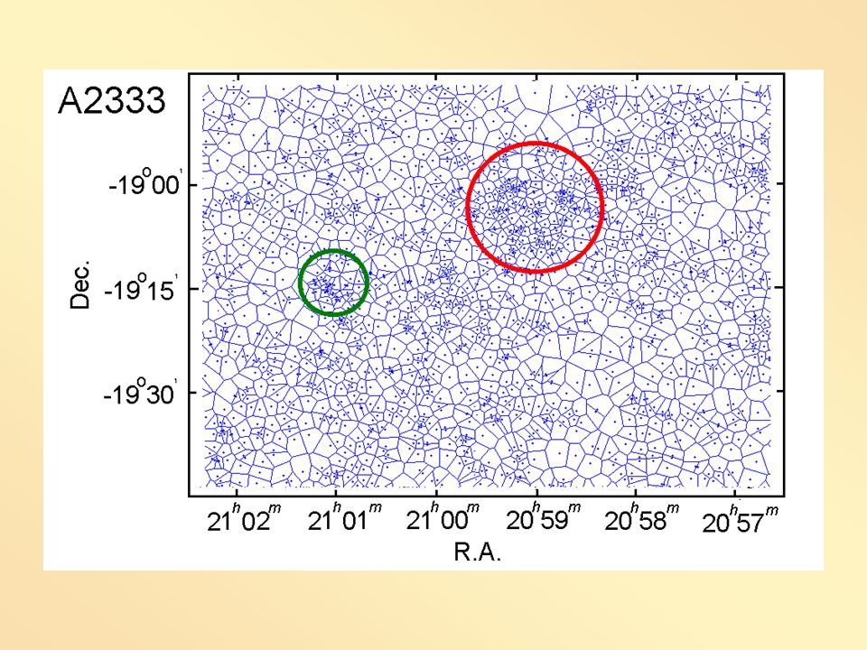
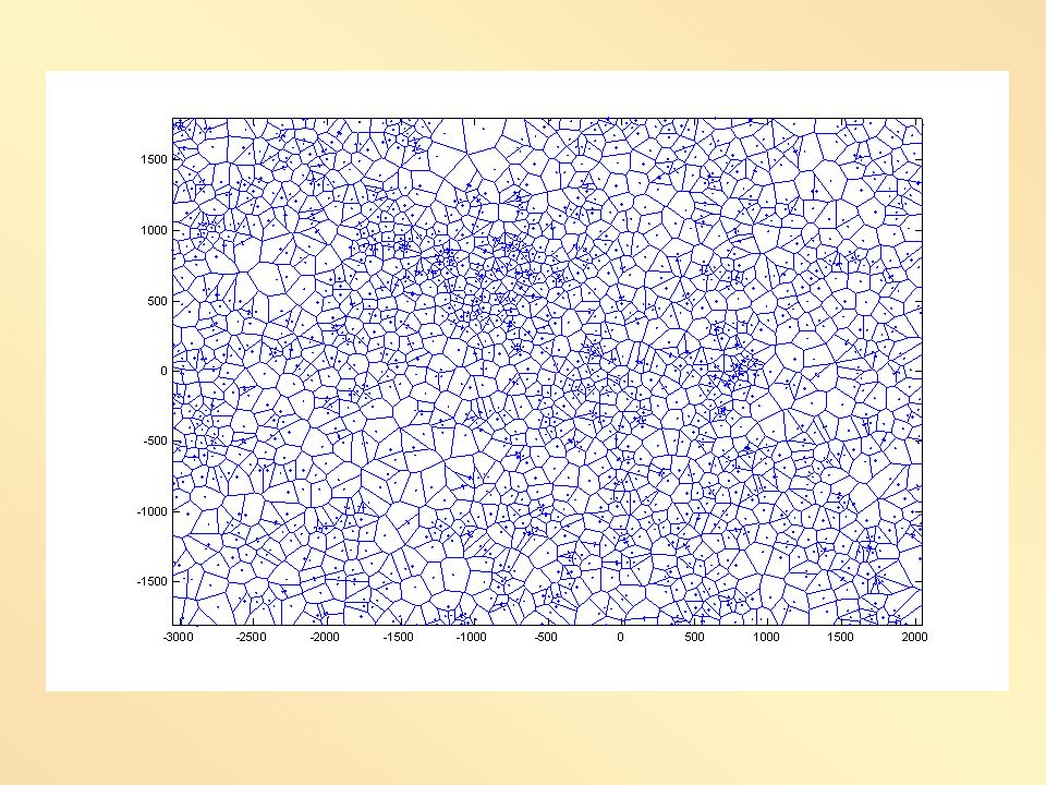
41 Structure finding We selected the Voronoi tessellation technique (VTT hereafter) for cluster detection. This technique is completely non-parametric, and therefore sensitive to both symmetric and elongated clusters, allowing correct studies of non-spherically symmetric structures. For a distribution of seeds, the VTT creates polygonal cells containing one seed each and enclosing the whole area closest to the seed. This is the definition of a Voronoi cell in 2D.

42

43

44 Structures PF and PF in tangential coordinates, north is up. Open dots represented the structure members, black symbols corresponded to brightest galaxy in cluster, and line notes the direction of fitted ellipse major axe. Ellipticity and major axis position angle are shown in the right corner for each structure. PJF 2009, AJ 138, 1709

45 Using standard covariance ellipse method for galaxies in the considered region within the magnitude limit m3, m3+3m, we determined the moments of the distribution: The semiaxes in arcsec for the best-fitting ellipse were calculated from: Ellipticity: Position angle:

46 Voronoi cells for PF region (left panel) and the found cluster members as black dots with non-clustered galaxies as open symbols (right panel). PJF 2009, AJ 138, 1709

47

48 Struktury PF 6188 struktur przedział jasności: m3 – m3+3m

49

50 PF JAD 2,1 (2006)

51

52

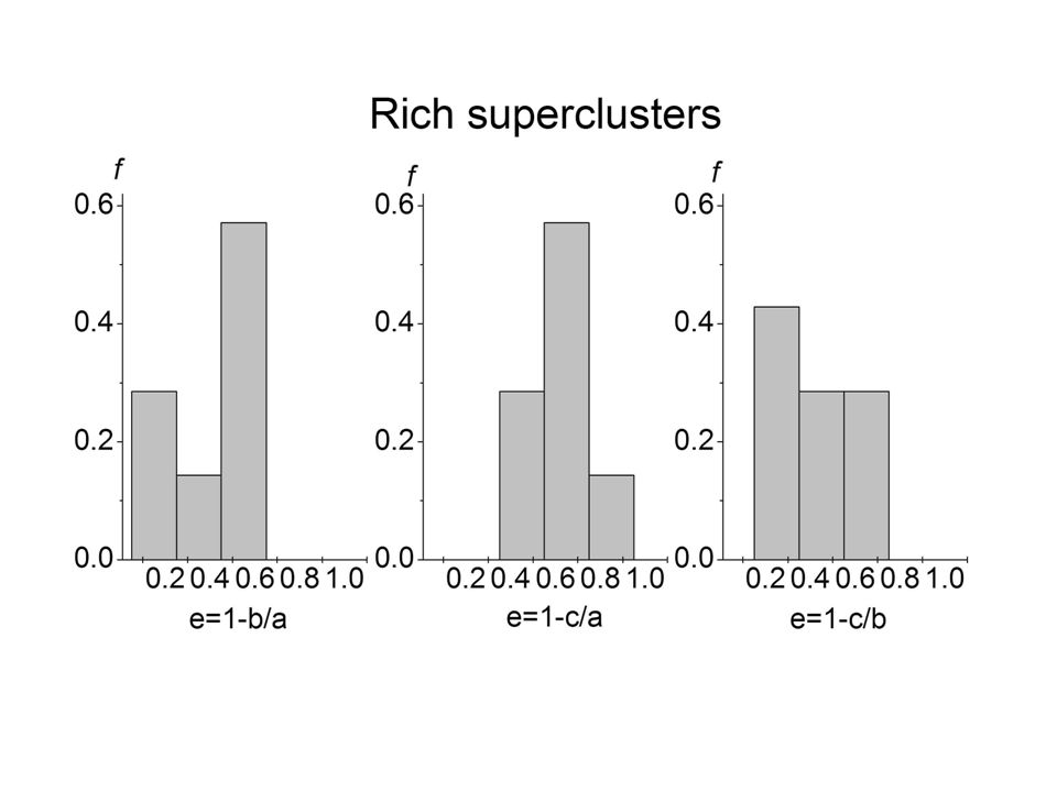
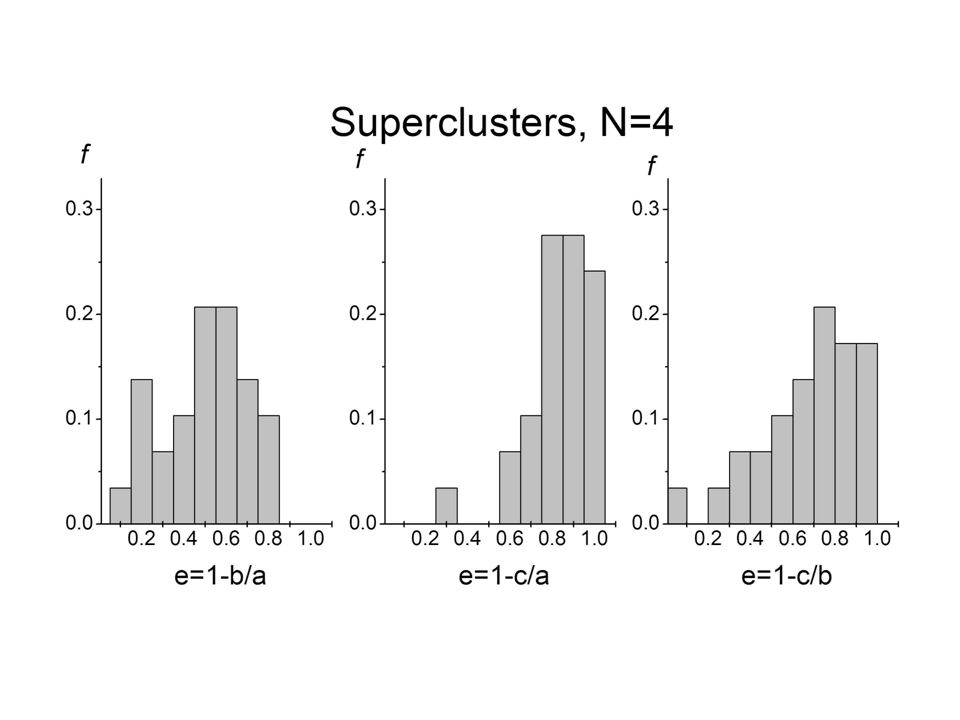
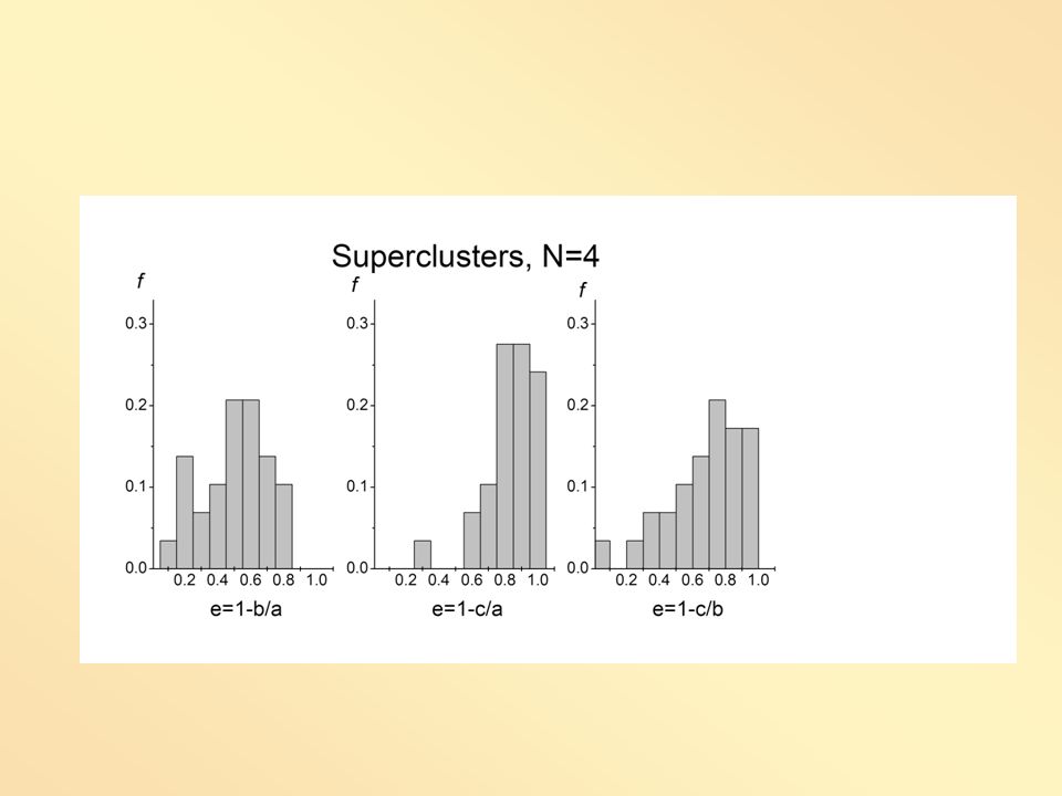
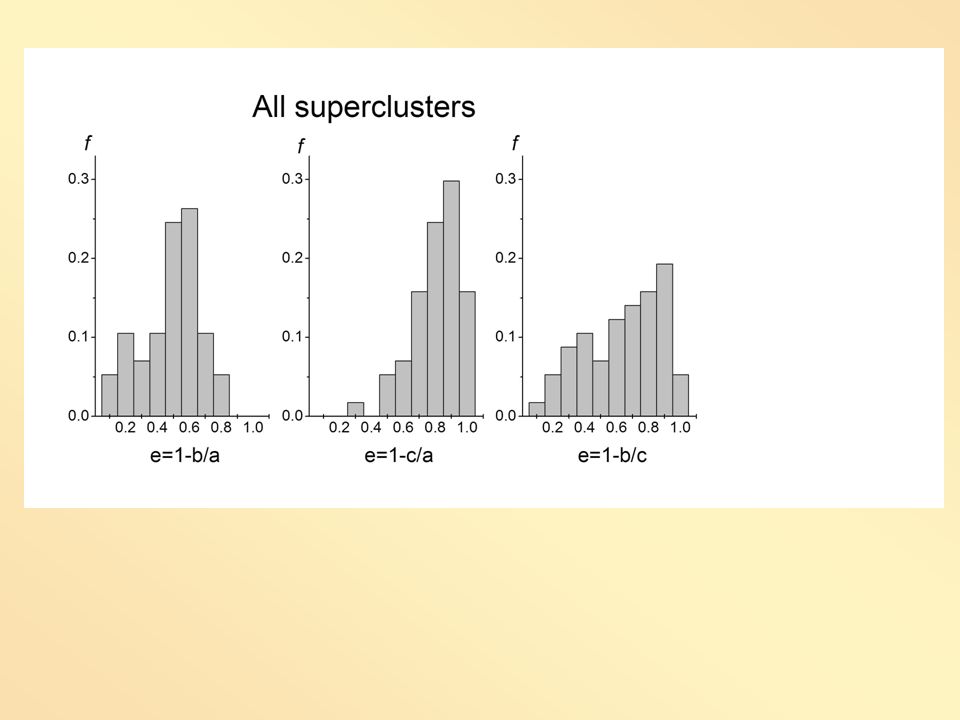
53 Results: very rich superclusters : Superclusters n=8 n>4
Angle P random Angle delta d: anisotropy Angle eta h: anisotropy In very rich clusters anlignment should be the greatest, if orientation ioriginated simultulanously with protostrcutures.. Anisotropy is increasing with structure size ( mass). The increase of anizotropii with richness was observed in the case of rich ( n>100) structures PF. Here the same pattern is confirmed.utaj jest potwierdzony.

54 Conclusions: Galaxy groups formed first, next they merge due to hierarchical clustering and formed greater structures. The protomain plane of the protostructure forms, which attracts other groups. Therefore structures are flat. This tendency is observed in the case of 1D i 2D structur.es Of course, this is preliminary results, which should be confirm on much bettter statistical sample.

55 Thank you for your attention

56

57

58 Orientation of the galaxy groups in the Local Supercluster
Piotr Flin, Włodzimierz Godłowski Institute of Physics, Jan Kochanowski University, Kielce, Poland Institute of Physics, Opole University, Opole, Poland

59 Recent dynamical evolution
Plionis (2002)

60 6068 struktur PF

61 The distribution of estimated z and the limits of the division into groups
BFJP 2009, ApJ 696, 1689

62 BFJP 2009, ApJ 696, 1689

63

64 BFJP 2009, ApJ 696, 1689

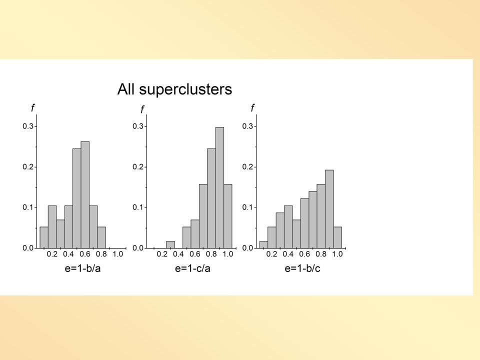
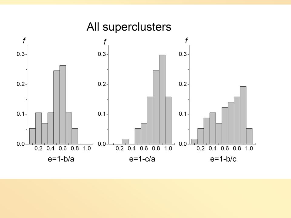
65 richness identified in the upper right portion of each section
The frequency distributions of structure ellipticities in four classes with richness identified in the upper right portion of each section (left panel all data, right panel 457 structures with m3+3m18m.3). PJBF 2009, ApJ 700, 1686

66 The frequency distribution of structure redshifts for
samples containing different number of galaxies in the structure (left panel all data, right panel 457 points) PJBF 2009, ApJ 700, 1686

67 The dependence of group richness on redshift z.
(left panel all data, right 457 points) PJBF 2009, ApJ 700, 1686

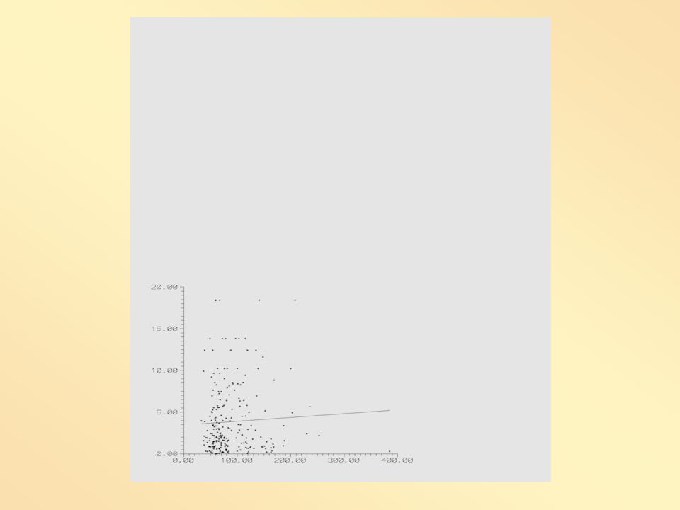
68 The ellipticity-redshift relation for galaxy group samples,
with the galaxy populations of each structure noted in the upper right hand corners. The fitted linear relations together with their = 0.95 confidence intervals are also plotted. PJBF 2009, ApJ 700, 1686

69 The cluster ellipticity e (left panel) and cluster ellipticity evolution rate de/dz ( right panel) versus redshift for four samples of different richness. Error bars correspond to  = 0.95 confidence intervals. (upper panel all data, lower 457 points) PJBF 2009, ApJ 700, 1686

70 Rozkład eliptyczności dla struktur z N>50 jest identyczny
Mniej spopulowane struktury są bardziej wyciągnięte niż bogate Małe grupy powstają na filamencie i następnie drogą hierarchicznego grupowania się powstają duże struktury, bardziej sferyczne. Dodatkowy argument za tym obrazem (średni redshift dla grup jest większy niż dla gromad) Relacja e-z zależy też od liczebności struktury. Eliptyczność małych grup i tempo ewolucji de/dz różnią się na poziomie 3 od tychże dla bogatych struktur Tylko struktury mające członków wykazują silną korelację e –z.. Numeryczne symulacje w ΛCDM dla z <3.0 wskazują, ze eliptyczność rośnie z przesunięciem ku czerwieni, jak też masą gromady. Potwierdzamy pierwszą tendencję, ale bardzo różne z, drugiej nie, ale w symulacjach bardzo masywne gromady 21013 h-1 Msłońca .

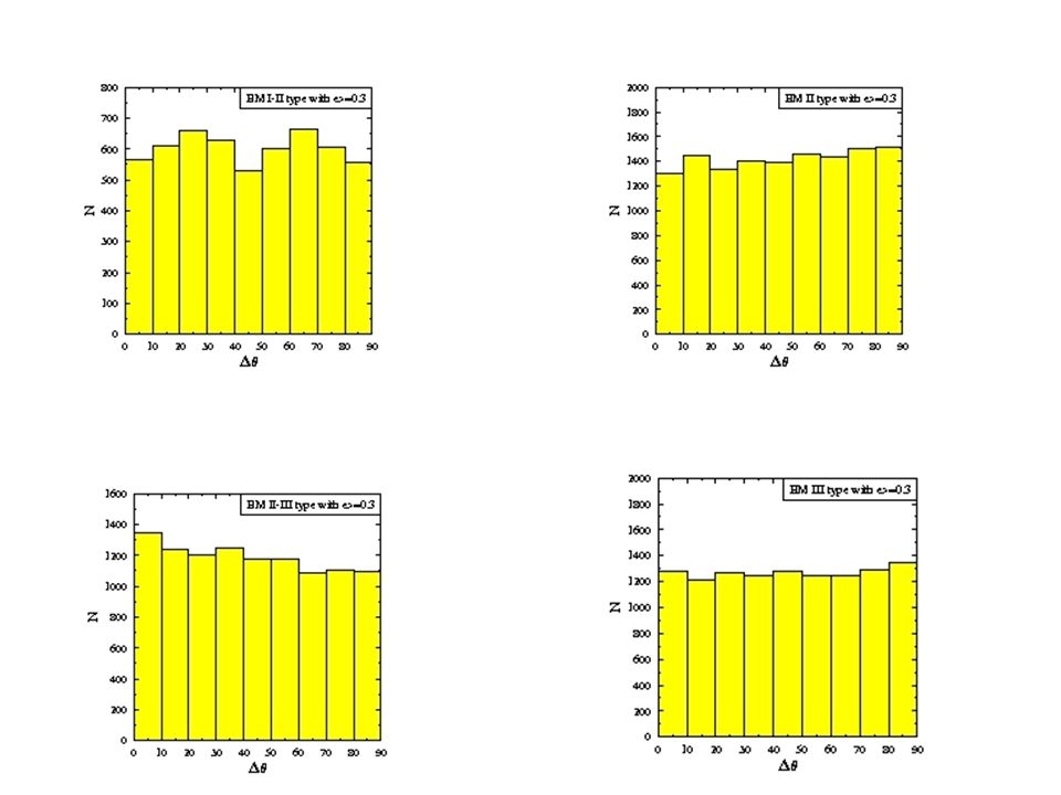
71 The division of ACO clusters corresponding to PF structures according
Type All 100 50-99 30-49 10-29 I 105 34 38 22 11 I-II 223 50 82 63 28 I-II: 8 4 1 2 II 55 72 59 37 II: 5 13 7 9 II-III 229 65 III 220 48 62 76 III: 14 3 1056 248 331 299 178 The division of ACO clusters corresponding to PF structures according to structure richness and B-M morphological types. PJF 2009, AJ 138, 1709

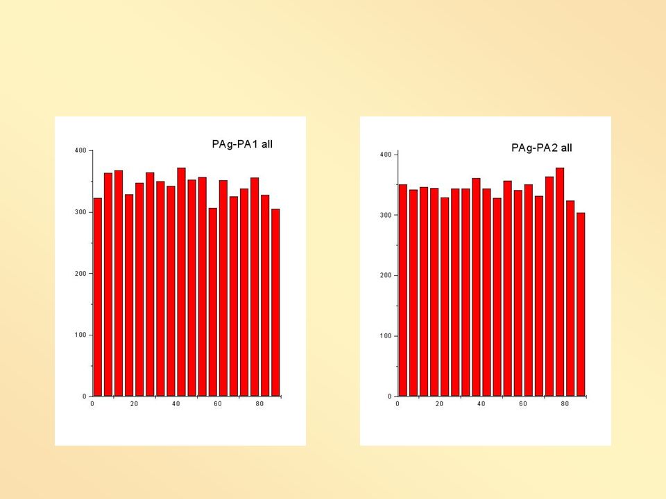
72 The frequency distribution of position angles for the two brightest galaxies PA1 and PA2 in the structure and structure position angle PAs. Dotted lines refer to an isotropic distribution, and a 1 error bar is also shown. PJF 2009, AJ 138, 1709

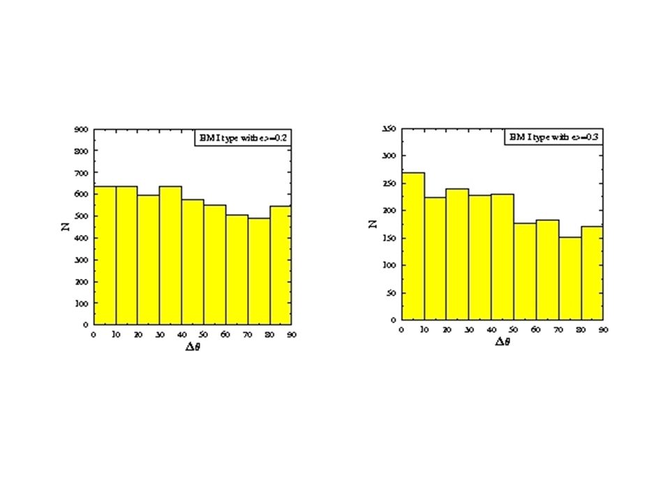
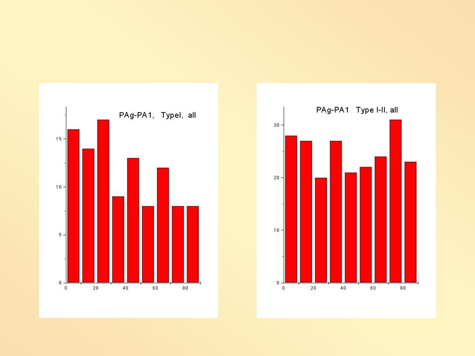
73 The frequency distribution of the angle θ1 between the brightest galaxy and parent cluster for groups of BM type I and I-II. Dotted lines show the isotropic distribution, together with a 1 error bar. PJF 2009, AJ 138, 1709

74 Brak orientacji galaktyk w gromadach jest zgodny z CDM
Procesy fizyczne w filamencie: albo Anizotropowe zlewanie się struktur (anisotropic merging + infall of matter) orientacja galaktyk Oddziaływanie przypływowe ( tidal torque) brak orientacji Nasz wynik: brak orientacji Galaktyki uzyskują moment pędu przez oddziaływanie przypływowe sąsiadów we wczesnym wszechświecie. Przepływ materii wzdłuż filamentu powoduje współliniowość najjaśniejszej galaktyki z dużą półosią gromady.

75 Efekt Binggeli’ego

76

77

78 Badanie Lokalnej Supergromady

79 Kąty pozycyjne : Pag kat pozycyjny grupy Pabm kat pozycyjny najjaśniejszej galaktyki Pal kat pozycyjny linii łączącej dwie najjaśniejsze galaktyki w grupie najjaśniej Pav kat pozycyjny na Virgo (kierunek na Virgo ) badano izotropię rozkładów tych 4 kątów Różnice kątów : Pag – Pav Pal – PaV Pag – Pal Pabm – Pag Pabm – Pal Pabm – Pav

80 GF ApJ 70,.920 (2010)

81

82

83

84

85 Różnice kątów Różnice kątów GF ApJ 70,.920 (2010)

86 Efekt Binggeli’ego dla grup
GF ApJ 70,.920 (2010) GF ApJ 70,.920 (2010)

87 Dwie najjaśniejsze galaktyki powstają na filamencie skierowanym do centrum LSC.
Poprzez oddziaływanie grawitacyjne grupy galaktyk powstają wzdłuż tej linii łączącej dwie najjaśniejsze galaktyki. Dlatego obserwuje się współosiowość kąta pozycyjnego struktury i linii łączącej dwie najjaśniejsze galaktyki.

88

89

90

91

92

93 Dziękuję za uwagę

94 Contingency table 0.05=1, 358 0.01=1.627 21-30 31-40 41-50 51-60
61-70 71-80 81-90 91-100 >100 10-20 3,7354 6,2565 7,2929 6,6493 6,1754 5,7794 4,5407 4,4379 7,4503 3,1015 4,5013 4,6979 4,5504 4,9033 3,0930 3,8179 6,3343 1,6189 2,4571 2,5490 3,1751 1,6852 2,6718 3,8782 1,3196 1,5201 2,2652 0,9619 2,0691 2,5903 0,6179 1,1031 0,1750 1,2746 1,0271 0,8063 0,2955 1,0595 0,8441 0,8065 0,4377 0,2852 1,0573 0,6658 90-100 0,6831 0.05=1, 358 0.01=1.627

95 PA Distribution The division of ACO clusters corresponding to PF structures according to structure richness and B-M morphological types Type All 100 50-99 30-49 10-29 I 105 34 38 22 11 I-II 223 50 82 63 28 I-II: 8 4 1 2 II 55 72 59 37 II: 5 13 7 9 II-III 229 65 III 220 48 62 76 III: 14 3 1056 248 331 299 178

96

97

98 In order to check the distribution of galaxy orientation angles (, ) and position angles p, we tested whether the respective distribution of the ,  or p angles is isotropic. Below, a short summary is presented of the tests considered here (not always explicitly): the 2-test, the Fourier test and the auto-correlation test. In all of these tests, the entire range of the  angle (where for  one can put +/2,  or p respectively) is divided into n bins, which in the 2 test gives n-1degrees of freedom. During the analysis, we used n = 18 bins of equal width. Let N denote the total number of galaxies in the considered cluster, and Nk - the number of galaxies with orientations within the k-th angular bin. Moreover, N0 - denotes the average number of galaxies per bin and, finally, N0,k - the expected number of galaxies in the k-th bin. The 2-test of the distribution yields the critical value 27.6 (at the siginificance level  =0.05) for 17 degrees of freedom: However, when we consider individual clusters the number of galaxies involved may be small in some cases, and the 2 test will not necessarily work well (e.g. the 2 test requires the expected number of data per bin to equal at least 7. As a check, in a few cases we repeated the derivations for different values of n, but no significant differences appeared. However, the main statistical test used in the present paper is the Fourier test. In the Fourier test the actual distribution Nk is approximated as: (we take into account only the first Fourier mode).

99 We obtain the following expression for the coefficients ij (i,j = 1, 2):
with the standard deviation where N0 is the average of all N0,k. However, we should note that we could formally replace the symbol  with = only in the cases where all N0,k are equal (for example, in the cases when we tested the isotropy of the distribution of the position angle).

100 The probability that the amplitude:
is greater than a certain chosen value is given by the formula: while the standard deviation of this amplitude is From the value of 11 one can deduce the direction of the departure from isotropy. If 11 < 0, then, for 2, an excess of galaxies with rotation axes parallel to the LSC plane is present. For 11 > 0 the rotation axes tend to be perpendicular to the LSC plane. Similarly, while analysing the distribution of the position angles of galaxies (p), if 11 < 0, an excess of galaxies with position angles parallel to the plane of the coordinate system (i.e. normal to the galaxy plane is perpendicular to the plane of the coordinate system) is present. For 11 > 0, the position angles of galaxy are perpendicular to the plane of the coordinate system.

101 The auto-correlation test quantifies the correlations between the galactic numbers in adjoining angular bins. The correlation function is defined as: In the case of an isotropic distribution we expected C = 0 with the standard deviation:

102 2

103

104 Statistical analysis indicates that structures containing more than 50 member galaxies appear to originate from the same parent population, in other words their structure ellipticity distributions are essentially identical. In agreement with earlier works (Struble & Ftaclas 1994, Plionis et al. 2004), it is found that the more poorly populated structures are more elongated than richly populated ones. It is suggested that such a result may reflect variations in the initial conditions during structure formation (Biernacka et al. 2008). Small elongated groups appear to have formed along pre-existing filaments, and later become more spherical in shape as a result of hierarchical clustering. Such a conclusion is supported by the discovery that, in the sample of 6188 structures investigated here, the mean redshifts for galaxy groups are larger than the mean redshifts for richer clusters. The e-z relation depends upon richness as well, with the dependence being similar to the rate of evolution of ellipticity de/dz as a function of redshift z. For poorly populated groups both the ellipticity and the ellipticity evolution rate de/dz differ at a 3 level from results found for other, more richly populated, samples. A redshift of z = 0.12 appears to divide the two samples. The sample containing galaxy aggregations containing between 10 and 30 members displays a significant correlation with redshift, while the three remaining samples for richer groups exhibit either a weak correlation or an anti-correlation. Recently, Plionis et al. (2009) investigated a sample of 150 ACO clusters with z < 0.14 containing at least 20 members. Their sample does not contain merging and interacting clusters, or clusters with dynamical substructures. They found that the direction of evolution is different for clusters of different richness. While their values of de/dz differ from the present results, the directions of the trends are identical. The differences that do exist can be attributed to the analysis of totally different samples, with different richness classes for the subsamples and different redshift limits. It has proven to be difficult to compare the present results with numerical simulations. A very extensive numerical study (Hopkins et al. 2005) in the framework of CDM cosmology examines cluster ellipticities to redshift z =3. The present study investigates low- edshift clusters, making a simple comparison impossible. The numerical simulations indicate that cluster mean ellipticity should increase with redshift as well as cluster mass. The present results agree with the first prediction, but conflict with the second. As pointed out above, however, the redshift coverage of our galaxy samples is very small in comparison with that of existing numerical simulations, and the simulations considered cluster masses of clusters greater than 21013 h-1M, which corresponds only to the richest of our samples.

105 The absence of alignment for brighter cluster galaxies is consistent with the CDM scenario of galaxy formation. There are two different, but not exclusive, points of view about the physical processes in filaments. One stresses the importance of anisotropic merging, the other tidal interaction (see e.g. Lee & Evrard 2007). In the naive prediction one can expect that the anisotropic merging and infall of matter along filaments will result in galaxies oriented non-randomly, while the action of tidal torques will produce a random orientation of galaxies. Our result supports the idea that galaxies formed in long filamentary structures. The lack of alignment of brighter galaxies points toward a process in which galaxies acquire angular momentum from tides exerted by their neighbours in the early Universe. On the other hand, the flow of matter along filaments causes the alignment of BCM galaxies with cluster long axes.

106 From the presented analysis of the orientation of galaxy groups in the Local Supercluster the
following picture of the structure formation appears. The two brightest galaxies were formed first. They originated in the filamentary structure directed towards the centre of the protocluster. This is the place where the Virgo cluster centre is located now. Due to gravitational clustering, the groups are formed in such a manner that galaxies follow the line determined by the two brightest objects. Therefore, the alignment of structure position angle and line joining two brightest galaxies is observed. The other groups are forming on the same or nearby filament. The flatness of the LSC additionally contributes to the observed alignment of galaxy groups. The majority of the groups lie close to us. Due to completeness of the Catalog, the lack of groups further than the Virgo Cluster centre is observed, but nearby groups are very well selected and they contain only more massive galaxies. This picture is in agreement with predictions of several CDM models, in which structure formation is due to hierarchical clustering. Moreover, the formation is occurring on the filamentary structure.

107 Wyobraźmy sobie sferę zawierającą masę całkowitą M w epoce rekombinacji (wszechświat jest bardzo jednorodny wtedy) . Niech < M/M> jest fluktuacją gęstości która wystąpiła wtedy w sferze poruszającej się losowo we wszechświecie. Wielkość < M/M> jest miarą niejednorodności Wszechświata.  Związek < M/M> z M zwana jest widmem fluktuacji gęstości (density fluctuation spectrum (DFS)). Jest to zależność fundamentalna . Matematyczny kształt tej funkcji opisuje wzrost struktur powstałych drogą grawitacji. Ponieważ po rekombinacji małe fluktuacje rosną liniowo jak (1 + z) -1, kształt DFS w momencie rekombinacji jest zachowany aż do momentu, gdy pierwsze z fluktuacji stają się nieliniowe. Gęstość wszechświata  zmienia się od miejsca do miejsca, a średnia gęstość to <>. Aby powstała struktura nadwyżka gęstości w danym miejscu opisana jako  / <> musi być wystarczająco większa od zera.

108 NIESTABILNOŚĆ GRAWITACYJNA
 Z tego warunku uzyskuje się dane o parametrach takich jak masa i amplituda. Są one dane prze index  i współczynniki normalizacji K i M0 widma mas.   / <> = k (M/M0)+  Index  jest związany ze wskaźnikiem widma mocy n zdefiniowanym przez (  / <>) 2 ~ l+n poprzez zależność:   = - ½ + n/6  Jeżeli jest funkcją czasu to widmo mas też.  Wydaje się, że  = - 2/3 wtedy perturbacje mają stałą krzywiznę kiedy docierają do horyzontu (n= -1). (Promień wszechświata jest ~ct). Gdy t = 1 rok masa wewnątrz 109 – 1011 MO .  ASTROPARTICLE PHYSICS EARLY UNIVERSE, GUT BOTH : VALUE OF  AS WELL TYPE OF PERTURBATIONS GENERATED IN THE EARLY UNIVERSE

109 Katalog struktur PF 6188 struktur , każda więcej niż 10 0 obiektów
W oparciu o ten katalog utworzono katalog supergromad Wiadmo, że supergromady są płąskie. Nasze badania to potwierdziły. Dlatego też porównanie w przypadku 2D robiono na supergromadach. Niestety nie jest to statystycznie ełna próbka, więc posłuzyła do badań wstępnych. Mamy 57 supergromad, z k tórych każda zawiera przynajmniej 4 struktury PF. Dla 257 bardzo bogatych gromad PF ( n>100) znamy rozkład kątów pozycyjnych oraz orietację osi rotacji. Sprawdzono, jak wygląda rozkład oso rotacji i kątów pozycyjnych bardzo bogatych gromad w supergromadach.

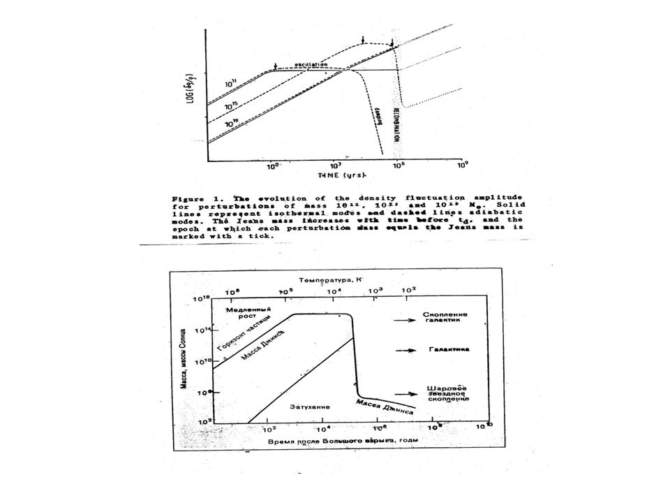
110 Nie ma możliwości bezpośredniego obserwowania początkowego widma mas, ewentualnie z wyjątkiem tylko dużych mas. Jest to wynikiem tego, iż wiele fizycznych procesów wpływało na perturbacje we wczesnym Wszechświecie. Niektóre z tych procesów są zależne od masy, inne nie. W epoce promieniowania amplituda fluktuacji gęstości o długościach fali mniejszych niż horyzont kosmologiczny pozostaje niezmieniona. Fluktuacje o większej długości fali niż horyzont rosną proporcjonalnie do czasu. Fluktuacje o coraz to większych długościach fali wchodzą w horyzont i ulegają zamrożeniu. Kiedy gęstości energii: promieniowania i materii stają się równe (zeq  2.5 x 104  h2 ) wszystkie perturbacje gęstości mogą rosnąć. Widmo mocy dla małych liczb falowych (czyli dużych długości fal) pozostaje niezmienione, dla małych długości fal szybko maleje do zera. Rozważmy perturbacje : 1011, 1015, MO . (masa galaktyki, masa największego skupiska gdzie  / <> >1 , oceniona przybliżonej masy Wszechświata w momencie oddzielenia (decoupling)) materii i promieniowania.

111

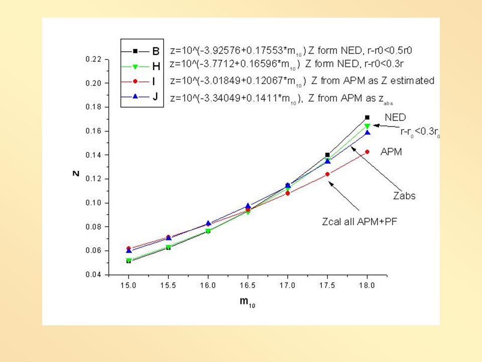
112 Table 1. The result of the statistical analysis of m10 - z relation
Identification for input data a b Number SD R 1 ACO (0.5r) -3.895 (±0.210) 0.1737 (±0.012) 455 0.17 0.56 2 ACO (0.3r) -3.771 (±0.242) 0.1660 (±0.015) 290 0.55 3 APM (0.5r) -3.813 (±0.148) 0.1684 (±0.009) 372 0.11 0.65 4 ACO (m10<19m.3) -3.767 (±0.195) 0.1641 (±0.0116) 519 0.18 0.28 BFJP, 2009, ApJ 696, 1689

113 Konkluzje Rozkład eliptyczności struktur zależy od liczebności struktury. Bardziej liczne – bardziej sferyczne. Zależność e(z). W przeszłości silniejsze oddziaływanie. Rozkłady kątów pozycyjnych dla 10 najjaśniejszych galaktyk – losowe. Różnice kątów pozycyjnych struktury i najjaśniejszych galaktyk – losowe. Tylko w przypadku gromad zawierających nadolbrzymią galaktykę cD obserwuje się współosiowość. Specjalna ewolucja tych gromad galaktyk. Struktury powstają na filamencie.

114 The distribution of structure ellipticity is identical for structures with N>50 members.
Less populated structures are more elongated than rich ones.  The small groups are forming on the filament and later on, due to hierarchical clustering, greater, more spherical structures are formed. The additional argument for this picture: the mean group redshift is greater than clusters. The elipticity – redshift realtion depends on the structure richness. The difference between ellipticity and evolution rate de/dz for small groups are at the 3 level different from rich ones. Only groups with member galaxies exhibit the strong e-z correlation. Numerical simulations show that in ΛCDM for z <3.0 ellipticity increases with z, as well as the structure mass. We support the first point, but our redshits are small. Simulation: very massive structures were considered (21013 h-1 Msun ).

115

116 Rozkład materii we Wszechświecie ( wielkoskalowa struktura):
Kosmiczna sieć ( pajęczyna) bardzo wydłużone struktury włókniste ( filaments) płaskie struktury ( ściany) (sheets, walls) gęste zwarte gromady galaktyk otoczone przez prawie puste obszary (pustki, voids) Topologia tych obszarów: Filaments (1D) Sheets (2D) Przechodzenie od obszarów pustych do pustych : przekraczanie ścian, czy jak w gąbce