Pobierz prezentację
Pobieranie prezentacji. Proszę czekać

1
Twój Partner w kontroli maszyn.

2
Strategia SPM

3
Jak przedstawiać system aby rzeczywiście był praktyczny ?
Światło czerwone : Niebezpieczeństwo Światło żółte: Ostrzeżenie Światło zielone: Cały system naprzód Inne techniki dają nieopracowane dane. SPM idzie krok naprzód, poprzez przygotowane odpowiedzi.

4
Sygnał częstotliwosciowy
Sygnał czasowy Sygnał częstotliwosciowy Frequency domain The frequency domain is described by the vibration spectrum.

5
? Energia Drgań 99 % siły związane z ruchem obrotowym 0.9 %
z udarami 0.1 % z tarciem ?

6
Parametry Stanu Siły Parametr Jednostki drgań stanu pomiarowe
Ruch VEL mm/s RMS obrotowy ACC mm/s2 RMS Udary CREST -- KURT -- SKEW -- Tarcie NL 1 m/s NL 2 ” NL 3 ” NL 4 ”

7
Parametry określające siły udarów
Dla sygnału “A” CREST = KURT = –1.244 SKEW = Dla sygnalu “B” CREST = KURT = –0.227 SKEW = Dla sygnalu jak w przypadku “B” lecz z symetrią względem osi x CREST = KURT = –0.227 SKEW = –0.31 Dla funkcji sinus: CREST = 1.414 KURT = –1.500 SKEW = 0.000 A B KURT SKEW CREST v peak –3 ( ) t – 3 s 1 n S ~ 4 RMS
 t. – 3. s. 1. n. S. ~ 4. RMS.")
8
Trendy i limity alarmowe
• Niewywaga • Niewyosiowanie • Luzy • Zużycie zmęczeniowe • Uszkodzenie kół zębatych • Inne uderzenia • Trące części • Film smarny VEL ACC CREST KURT SKEW NL1- 4

9
Kryteria kolorowej oceny sygnału
Numer COND czerwony powyżej 5 jednostek żółty pomiędzy 3 i 5 jednostek zielony do 3 jednostek czas mm/s Obliczenia statystyczne

10
Ocena stanu 60 50 40 30 20 10

11
Parametry oceny stanu 60 50 40 30 20 10 Rotational forces Vel Acc
Rotational forces Vel Acc Shock Crest Kurt Skew Friction NL1 NL2 NL3 NL4

12
Sygnał częstotliwościowy Sygnał czasowy
Frequency domain The frequency domain is described by the vibration spectrum.

13
Od zapisu w funkcji czasu do rozkładu drgań w funkcji częstotliwości
Sygnał w funkcji czasu ( mierzony sygnał drgań) jest rozkładany na funkcje sinusoidalne z pomocą analizy Fouriera FFT = fast Fourier transfer których amplitudy są kreślone w funkcji częstotliwości aby otrzymać spektrum drgań
 jest rozkładany na. funkcje sinusoidalne. z pomocą analizy Fouriera. FFT = fast Fourier transfer. których amplitudy są kreślone. w funkcji częstotliwości. aby otrzymać. spektrum drgań.")
14
Analiza widmowa drgań mm/s , mm/s , μm 2 Hz , cykle/min.

15
Typowa praca z analizą widma
Symptom Niewyosiowanie Zła współpraca kół zębatych

16
EVAM Evaluated Vibration Analysis Method â

17
Przyrządy Oprogramowanie Ocena EVAM®

18
Jakich uszkodzeń możemy się spodziewać ?

19
Typowe mechaniczne uszkodzenia
Niewspół - osiowość Powiększone luzy Niewłaściwe podparcie Uszkodzenie przekładni zębatej Niewyważenie Zniszczenie łożysk ( ok.80%)
")
20
Komponenty. 3: WAŁ ŁOŻYSKO SKF NJG2332 VH
(BPFO, BPFI, BPFIM, BSF, BSFM) KOŁO ZĘBATE Z63 (GM, GMMOD) Komponenty. 1:WAŁ ŁOŻYSKO SKF 32320 KOŁO ZĘBATE Z13 2:WAł ŁOŻYSKO SKF NCF 2944V KOŁO ZĘBATE Z36
 KOŁO ZĘBATE Z63. (GM, GMMOD) Komponenty. 1:WAŁ. ŁOŻYSKO SKF KOŁO ZĘBATE Z13. 2:WAł. ŁOŻYSKO SKF NCF 2944V. KOŁO ZĘBATE Z36.")
21
Symptomy.

22
Zaznaczone symptomy.

23
Wartość symptomu Pasmo wartość RMS = Symptom wartość RMS = v +
200 Pasmo wartość RMS = Symptom wartość RMS = Symptomy jako WARTOŚĆ lub COND v 1 2 3 + 4 5 6 7 v4 v2 v3 v5 v6 v7 v1 mm/s

24
SPM EVAM Dwie drogi do celu ® Kondycja Numer Łożyska Założenia
do pomiarów Objawy uszkodzeń Parametry objawów Kryteria stanu Kondycja SPM EVAM Dwie drogi do celu

25
Przygotowanie do pomiaru EVAM
Punkt pomiarowy Założenia do pomiarów Symptomy uszkodzeń Niewywaga Niewyosiowanie Łożysko Przekładnia zębata Drgania pasa BPFO BPFI BPFIM BSF BSFM FTF Przygotowanie do pomiaru EVAM

26
Dane wejściowe. SPM Natężenie drgań EVAM Komponenty Przybliżona
prędkość obrotowa Wielkość łożyska Natężenie drgań Klasa maszyny EVAM Komponenty Konstrukcja maszyny Dokładne dane Statystyka Dokładna RPM

27
Niewłaściwe podparcie
Metoda Natężenie Metoda SPM ® drgań EVAM ® Funkcje pomocnicze SPM Spectrum, Temperatura, Obr./min., Smarowanie, Przepływ, Ciśnienie, itp. Niewyważenie Niewspółosiowość Nadmierne luzy Niewłaściwe podparcie Np. Uszkodzenia przekładni zębatych Kondycja łożyska Stan smarowania

28
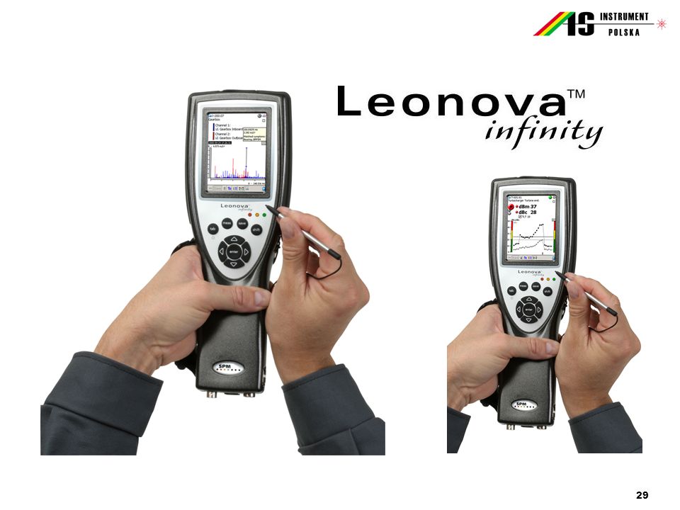
Analizator Stanu Maszyn A30 wersja EXPERT
Przyrządy wielofunkcyjne : Analizator Stanu Maszyn A30 wersja EXPERT

30
Leonova A30 Porównanie z poprzednimi przyrządami - funkcje Expert
SPM Spectrum Porównanie z poprzednimi przyrządami funkcje Leonova Wyważanie 2-płaszczyznowe Wyważanie 1-płaszczyznowe EVAM – automatyczna analiza FFT Metoda SPM do łożysk ISO 10816 Temperatura Basic Logger Expert A30 Pomiary alternatywne Kontrola punktów pomiarowych Osiowanie poziome i pionowe

31
CMS- System kontroli ciągłej.
Moduły VCM

32
Condmaster® - łatwe w obsłudze oprogramowanie.
• SPM® • VIB • EVAM® • Temperatura • R.P.M.( obr/min ) • Zdefiniowane przez użytkownika • Kontrola
 • Zdefiniowane przez. użytkownika. • Kontrola.")
33
Zniszczenie łożyska FIRMA … HALA … MASZYNA …

34
Graphics: results for one measurement
Graphics: results for one measurement. Click on a result (black square) to open. All active parameters and symptom values are shown, but no RPM value.
 to open. All active parameters and symptom values are shown, but no RPM value.")
35
Graphics: ”Measuring results” active
Graphics: ”Measuring results” active. The last result shown graphically is at the top of the list. Pull the lower edge to extend the list.

36
Measuring point: Deactivate the symptom 20 Gear damage for the 200 Hz assignment. It is outside of the frequency range.

37
Measuring point: Once measuring results are recorded in Condmaster Pro, the condition parameters and the symptoms should be edited in the measuring point register. Deactivate those which do not add to the condition information. ACC normally gives the same information as VEL. Keep VEL for comparison with the symptom values. KURT normally produces the same diagram as CREST. Keep CREST. SKEW is very difficult to interpret and normally deactivated. The 5000 Hz assignment covers the range needed for symptom 20 Gear damage, but gives a very poor resolution for all other symptoms. Deactivate systems 10, 60, 61 – they are covered by the 200 Hz assignment. Thus you reduce the number of graphs, which makes it easier to check the essential condition information.

38
Symptom: Check the symptom configuration
Symptom: Check the symptom configuration. 20 Gear mesh Z1 looks for gear mesh modulation on the ingoing shaft. Z1 is the number of gear teeth, RPM1 the rpm of the ingoing shaft. The centre frequency is not included. This is the actual gear mesh frequency, which is normally always seen in the spectrum, even when the gear is in good order. The sidebands are the damage indicators. Three sidebands means six lines. With four harmonics, the total number of symptom lines is 24.

39
Podświetlanie symptomu

40
Spectrum: A spectrum is difficult to read unless one can highlight significant lines. Use the functions under ”...” when working with the spectrum.

41
Spectrum: Matching lines marked in yellow, here the gear mesh frequency with rpm modulation, three sidelines, no centre line, four harmonics. Each harmonic thus includes 6 lines, making 24 for the whole symptom. Of these, 21 have been found in this spectrum (Match 21). The total velocity value of these 21 lines is 0.34 mm/s. Compare this with the RMS value VEL = 1.81 mm/s. This symptom contains less than 20% of the measured RMS value.

42
Spectrum: ”Theoretical symptom” marks the position of all symptom lines in blue. The symptom 20 Gear damage Z1 is the gear mesh frequency with rpm modulation, three sidelines, no centre line, four harmonics. Each harmonic thus includes 6 lines, making 24 for the whole symptom. The program found 21 matching lines out of this 24, with a total amplitude value of 0.34 mm/s.

43
Spectrum: Dragging the cursor over a part of the spectrum zooms in on this section. This cannot, of course, change the resolution of the spectrum, but produces an enlarged picture on the screen.

44
Spectrum: Below the spectrum on the right hand side, two values show the present position of the cursor, horizontal in Hz and vertical in mm/s. Thus, one can read off the position and amplitude of any line by simply moving the cursor and without marking the line.

45
Spectrum: the function ”Show harmonics” projects harmonics of the marked line as red dotted lines onto the spectrum. Here, the unbalance symptom line at 1X is marked. ”Show harmonics” can be used to find out whether lines with high amplitude, apparently not matching any probable symptom, belong to a pattern. In this case there are no significant harmonics, only two matching lines with low amplitudes (here marked with white squares).
.")
46
Ringing: The SPM test rig is a very small machine on a fairly elastic metal frame. The response varied considerably, depending on which part was struck: the frame, the gearbox, the pump.

47
”Compare spectrum”, when selected from the Graphic Evaluation, shows the spectra for all measuring points visible in the marked diagram. Use this function to check whether the same line or patters of lines are consistent for the whole group of spectra.

48
Ringing: The readings were taken with the long-time recording function of a T30. Here are part of them shown by ”Compare spectrum”. Another worthwhile experiment is to start a long-time recording of speed and EVAM, then shut off the machine power. Check the VEL graph for high values, then use the spectrum to find the frequencies that fall into areas of machine resonance. The areas of resonance are stable, independent of the RPM. All symptoms having an RPM variable will move towards the lower end of the frequency range as the RPM goes down. When it coincides with a resonance area, the symptom line amplitude should go up.

49
www.asinstrument.com.pl www.asinstrument.eu
Do usług ... 71537Y © Copyright SPM Instrument AB

Podobne prezentacje


-e*h*(k*o-l*n))+f*i*j*n>")


 strugi v=0,>")
